6 Tips to Make a High-Quality Spreadsheet on Excel or Google Sheets
Creating a spreadsheet? These hacks will make your work pop.


- She received the Renau Writing Scholarship in 2016 from the University of Louisville's communication department.

There are dozens of reasons to make a spreadsheet like business presentations, school presentations, budgeting, habit-tracking, book-tracking and managing the kids' chores. But how do you make your spreadsheet pop for that special meeting? How do you make Google Sheets or Excel work for you, and not the other way around?
These programs are packed full of useful features, as well as shortcuts to work smarter, not harder.
Here are six tips to turn you into a spreadsheet pro whether you're using Microsoft Excel or Google Sheets.
Alphabetize your data
You can customize your spreadsheet data a number of ways, including alphabetical -- or reverse alphabetical -- order.
Here's how for Google Sheets:
1. Highlight a column or click the capital letter at the top of the column.
2. Click the down arrow to open the dropdown menu.
3. Choose Sort sheet A-Z or Sort sheet Z-A. Note that sorting A-Z will also arrange numbers from lowest to highest, and sorting Z-A will arrange them from highest to lowest.
Here's how for Excel:
1. Highlight a column
2. Click the Data tab
3. Click A-Z for alphabetical order or Z-A for reverse alphabetical order.
Add checkboxes
Who doesn't love a to-do list? If you're using a spreadsheet for task completion or habit-tracking, checkboxes can be helpful.

Where to find checkboxes in Google Sheets
Here's how for Google Sheets:
1. Highlight a column, cell or row.
2. Click Insert in the toolbar
3. Choose Checkbox
Here's how for Excel:
1. Click Insert
2. Select the checkbox under Form Controls
3. Click the cell where you want to insert the checkbox and the box will appear for you to place when your cursor turns to a four-pointed arrow.
4. Highlight the column with the checkbox and drag your cursor down to the desired length.
Dropdown menus
For an extra polished spreadsheet, add dropdown menus.
Here's how to add for Sheets:
1. Highlight a column, cell or row.
2. Click Insert in the toolbar.
3. Click Dropdown.
The dropdown menu will default with two options, but you can further customize by clicking the edit icon.
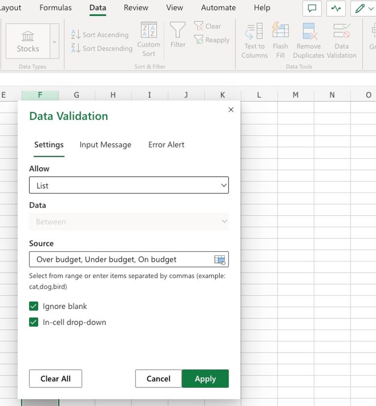
Adding dropdown menus in Excel.
Here's how to add for Excel:
1. Select the cells you want to add a dropdown menu to.
2. Click Data.
3. Choose Data Validation.
4. When the Data Validation pop up appears, select Allow.
5. Choose List from the menu.
6. Enter the content for your dropdown menu and separate each item with a comma.
7. Click OK.
Totaling a column
Data tracking usually involves a modicum of math, but drop that calculator, because there's an easier way to crunch numbers.
Here's how to add for Sheets:
1. Click into an empty cell.
2. Type =SUM(
3. Enter the range of data you want to total.
4. Add a close parenthesis.
5. The sum total will appear in the empty cell you originally chose.
You can also select a data range and Sheets will give you a preview in the bottom right. From there, you can change the sum, average, count and other functions.
Here's how to add for Excel:
1. Select the data range you wish to add together.
2. Check the status bar at the bottom of the screen.
3. You should see the total next to SUM.
You can achieve the same result using AutoSum, which will keep your total in your chart.
Charts
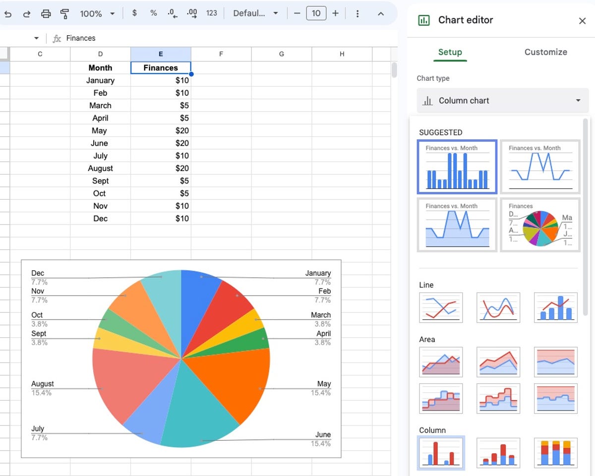
There are plenty of ways to customize your chart in Google Sheets.
A well-placed pie graph can really elevate a spreadsheet. And charts based on spreadsheet data will continuously update as you add more data.
Here's how to incorporate charts into your work in Google Sheets:
1. Enter the data you want to graph.
2. Highlight the columns.
3. Click Insert from the toolbar.
4. Click Chart in the dropdown menu.
5. A chart will populate and a side menu will open on the right side of your screen.
The customization menu lets you choose from options like different graph styles, colors and legend details.
Here are the steps for Excel:

Building a chart in Microsoft Excel
1. Select the data you want in your chart.
2. Click Insert.
3. Choose Recommended Charts.
4. Scroll through the options and click on a chart to see how it would display your data.
5. Click OK once you find the chart you want.
Explore the chart elements, styles and filters in the upper-right corner to further customize your chart.
Freeze columns or rows
If you're working with a large data set with lots of corresponding options, the less scrolling you have to do, the better. Freezing data in your spreadsheet means that the particular means that no matter how far you scroll, that first row or column won't move. It's particularly useful if your first row and column are titles for your x and y axis.
Here's how to freeze certain columns and rows on Sheets:
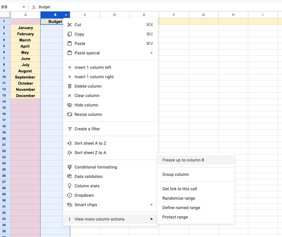
How to freeze columns and rows in Sheets.
1. Click the column that you want to remain stationary when you scroll through your data.
2. Click the down arrow in the corresponding column/row or right click.
3. Choose View More Column/Row Actions at the bottom of the menu.
4. Click Freeze Up to Column/Row [letter]. This will also freeze any columns or rows before the selected one.
Here are the steps in Excel:
1. Choose the row and column you want to freeze.
2. Click View.
3. Click Freeze Panes.
You can also freeze multiple rows and columns the same way.
For more information, check out how you can get Microsoft Word, Excel and PowerPoint for free, as well as how to turn a photo into an Excel spreadsheet.